Dissecting ML Models With NoPdb

I recently released NoPdb, a non-interactive (programmatic) Python debugger. This post, published in Towards Data Science, shows how to visualize attention in the Vision Transformer (ViT) with the help of NoPdb.

Motivation

Debugging machine learning models is very different from debugging “traditional” code. In deep neural networks, we have to deal with large feature maps and weight matrices which are usually meaningless to look at. With the increasing importance of ML interpretability, several methods for analyzing these internal representations have been devised, but in practice, obtaining them is not always straightforward. A classical debugger like Pdb may help, but using it for visualizations and analyses would be inconvenient to say the least.

While some frameworks like PyTorch address this by allowing to attach hooks to layers of a network, this only works in situations where the features we are interested in are available as the input or output of a particular layer. If we want to access information that is only available as local variables inside some function­ — for example attention weights in many implementations of the now omnipresent Transformers — we are out of luck.

Or are we?

Meet NoPdb

NoPdb (disclosure: I am the author) is a non-interactive Python debugger. Unlike Pdb, the standard Python debugger, NoPdb does not have an interactive user interface, but can be programmed — using convenient context managers — to execute certain actions when a given piece of code runs. For example, we can use it to easily grab a local variable from the depths of someone else’s code and save it for later analysis, or even modify its value on-the-fly to see what happens.

The basic functionality that we are going to use here is provided by nopdb.capture_call() and nopdb.capture_calls() (see the docs). These context managers allow capturing useful information about calls to a given function, including arguments, local variables, return values and stack traces. An even more powerful context manager is nopdb.breakpoint(), which allows executing user-defined actions (e.g. evaluating expressions) when a given line of code is reached.

Dissecting a Vision Transformer

To see NoPdb in action, we will apply it to a Vision Transformer (ViT). ViT is a recently proposed image classification model based completely on the Transformer architecture. The main idea, illustrated below, is fairly simple: split the input image into patches, run each of them through a linear layer, then apply a standard Transformer encoder to this “patch embedding” sequence. To do classification, a common trick is used: we add a special [class] token at the beginning of the input sequence, and attach a classification head (a single-layer MLP) to the corresponding (first) position in the encoder output.

Vision Transformer (ViT).

While we don’t care that much about the details of the architecture in this post, we do need to know that each layer of the model contains an attention mechanism, which computes a weight (a sort of similarity score) for every pair of input positions (i.e. image patches, plus the [class] token). Visualizing these weights, as we will do now, can give us a clue about which parts of the image are most important for the model.

We will use a pre-trained ViT from the timm package from the pytorch-image-models repository, and we will be following this Colab notebook (the most important parts of the notebook are included here).

Running ViT

Let us first install the timm computer vision package, as well as NoPdb:

pip install timm==0.4.5 nopdb==0.1

Loading the pre-trained model is easy:

import timm
model = timm.create_model('vit_base_patch16_224', pretrained=True)
model.cuda()
model.eval()

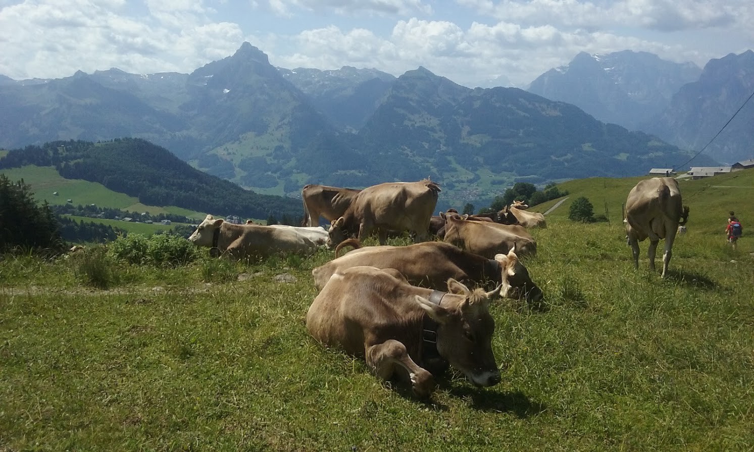
Now we will load an image and feed it to the model. Let’s try this photo I took in Switzerland:

Cows in Amden, Switzerland.

# Configure the pre-processing
from timm.data import resolve_data_config, create_transform
config = resolve_data_config({}, model=model)
transform = create_transform(**config)

# Load the image and pre-process it
img = PIL.Image.open('cows.jpg').convert('RGB')
input = transform(img).cuda()[None]

# Feed it to the model
model(input)

What the model returns are the logits (pre-softmax values) of all the classes. In the notebook, I wrote a small function, predict() , to print the most likely classes and their probabilities. Calling predict(input) gives:

alp     0.7936609983444214
ox      0.1110275536775589
valley  0.029854662716388702
oxcart  0.008171545341610909
ibex    0.008044715970754623

Visualizing the attention

Now let’s look inside the model! ViT consists of 12 blocks, each containing an attn layer; this is where the attention weights are computed:

VisionTransformer(
  (patch_embed): PatchEmbed(
    (proj): Conv2d(3, 768, kernel_size=(16, 16), stride=(16, 16))
  )
  (pos_drop): Dropout(p=0.0, inplace=False)
  (blocks): ModuleList(
    (0): Block(
      (norm1): LayerNorm((768,), eps=1e-06, elementwise_affine=True)
      (attn): Attention(
        (qkv): Linear(in_features=768, out_features=2304, bias=True)
        (attn_drop): Dropout(p=0.0, inplace=False)
        (proj): Linear(in_features=768, out_features=768, bias=True)
        (proj_drop): Dropout(p=0.0, inplace=False)
      )
      (drop_path): Identity()
      (norm2): LayerNorm((768,), eps=1e-06, elementwise_affine=True)
      (mlp): Mlp(
        (fc1): Linear(in_features=768, out_features=3072, bias=True)
        (act): GELU()
        (fc2): Linear(in_features=3072, out_features=768, bias=True)
        (drop): Dropout(p=0.0, inplace=False)
      )
    )
    ...
  (norm): LayerNorm((768,), eps=1e-06, elementwise_affine=True)
  (pre_logits): Identity()
  (head): Linear(in_features=768, out_features=1000, bias=True)
)

Let’s say we want to visualize the attention in the 5th block, i.e. model.blocks[4] . Looking at the code of the Attention layer, we can spot a variable called attn , which is exactly the attention tensor we’re after:

To get our hands on its value, we will use the nopdb.capture_call() context manager to capture the call to the attention layer’s forward method:

import nopdb

# The next line is where all the magic happens!
with nopdb.capture_call(model.blocks[4].attn.forward) as attn_call:
    predict(input)

And voilà — the attn_call object now contains a bunch of useful information about the call, including the values of all the local variables! Let’s see what they are:

>>> attn_call.locals.keys()
dict_keys(['self', 'x', 'B', 'N', 'C', 'qkv', 'q', 'k', 'v', 'attn'])

Inspecting attn_call.locals['attn'], we can see it’s a tensor with shape [1, 12, 197, 197], where 1 is the batch size, 12 is the number of attention heads, and 197 is the number of image patches + 1 for the [class] token (remember, the attention mechanism computes a weight for every pair of positions).

There are different ways we could analyze these attention matrices, but for the sake of simplicity, I chose to just visualize how much attention each patch is getting on average (for each attention head):

def plot_attention(input, attn):
    with torch.no_grad():
        # Loop over attention heads
        for h_weights in attn:
            h_weights = h_weights.mean(axis=-2)  # Average over all attention keys
            h_weights = h_weights[1:]  # Skip the [class] token
            plot_weights(input, h_weights)

(The helper function plot_weights, which just displays the image and adjusts the brightness of each patch according to its weight, can be found in the notebook.)

Calling plot_attention(input, attn_call.locals[‘attn’][0]) produces one plot for each of the 12 attention heads. Here are some of them:

Average attention weights in the 5th Transformer block (contrast increased for better viewing). The brighter each patch, the higher the attention weight.

We can see that some heads tend to focus mostly on a specific object in the image like the cows (head 8) or the sky (head 12), some look all over the place (head 2), and some attend mostly to one seemingly random patch like a part of a mountain in the background (head 3).

Please keep in mind that this is just a limited example. We could take this a step further by using attention rollout or attention flow, which are better ways of estimating how individual input patches contribute to the output, and we would be able to take advantage of NoPdb in pretty much the same way.

Tweaking the weights

Another thing NoPdb can do is “insert” code into a function. This means we can not only capture variables, but also modify them! I picked a somewhat silly example to demonstrate this: we are going to take the pre-softmax attention weights in all layers and multiply them by 3. (This is like applying a low softmax temperature, which makes the distribution more “peaked”.) We could of course do this by editing the code of the timm package, but we would then need to reload the package and the model, which can be tedious, especially if we need to do it repeatedly. NoPdb, on the other hand, allows us to do changes quickly, without any reloading.

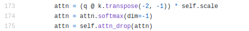
Let’s take another look at Attention.forward():

We would like to put attn = attn * 3 just before the softmax, i.e. on line 174. We are going to do this by setting a “breakpoint” at this line and making it execute this statement. (Note that a NoPdb breakpoint does not actually stop the execution; instead, it just executes some code that we give it.) We are also going to capture the local variables of the 5th block just like before.

# Set a breakpoint in the Attention module, just before the softmax
with nopdb.breakpoint(function=Attention.forward, line='attn = attn.softmax(dim=-1)') as bp, \
     nopdb.capture_call(model.blocks[4].attn.forward) as attn_call:
    bp.exec('attn = attn * 3')  # This code will get executed whenever the breakpoint is hit
    predict(input)

Note that we are not specifying the line number (174), but the actual code at that line: line='attn = attn.softmax(dim=-1)'— this is just a convenience feature, and line=174 (as in a classical debugger) would work as well. Also, note that since we specified the function as Attention.forward (and not model.blocks[4].attn.forward, for example), the breakpoint will get triggered at every single attention layer.

Let’s see how this changes the predictions:

balloon     0.2919192612171173
alp         0.12357209622859955
valley      0.049703165888786316
parachute   0.0346514955163002
airship     0.019190486520528793

And the attention patterns we captured:

A note on other frameworks

Although this post focuses on PyTorch, NoPdb does not depend on any particular framework and can be used with any Python 3 code.

That said, some frameworks, such as TensorFlow or JAX, compile models into computational graphs or directly into compute kernels, which are then executed outside Python, inaccessible for NoPdb. Luckily, in most cases we can disable this feature for debugging purposes:

• In TensorFlow 2.x, we can call tf.config.run_functions_eagerly(True) before executing the model. (Note that this will not work with models written for TensorFlow 1.x, which are explicitly compiled into graphs.)
• In JAX, we can use the disable_jit() context manager.

Some NoPdb links

• Colab notebook for this post
• GitHub repository
• Docs